This post follows, more or less, the content of a talk I gave at the BBVA Fundation in Madrid in April 2019. You can see the video (in Spanish, with English captions provided by YouTube’s Autotranslate) or you can check out the slides.

In 2013, I was attending a workshop on noise, information and complexity at the Ettore Majorana Center in beautiful Erice, Sicily, a medieval town sitting on top of a steep hill overlooking the western part of the island. The town, a network of tiny, winding streets lined mostly with medieval buildings, was foggy most days. The Center I was visiting, apart from its awe-inspiring location, is said to have played an important role in fostering relationships between scientists of the West and the East during the Cold War. As a proof of its openness to hosting even the most unexpected of visitors, the Center proudly displays a picture of Pope John Paul II seated behind a version of Dirac’s equation missing an all-important 

(Credit: Ettore Majorana Center)
One afternoon, the hosts of the workshop drove us down to Palermo for sightseeing. We toured a number of churches, whose layered styles and decorations reflected the different cultures that flourished on the island over the centuries. The last stop on our tour was the Martorana Church, an Italo-Albanian church of the 12th century, where to this day Mass is held in ancient Greek (yes, it is a complicated history). And while everybody had their noses up in the air, admiring the golden mosaics on the ceilings and the late baroque decorations, I was mesmerized by what lied underneath my feet. I am not talking about some forgotten crypt or creepy burial vault: I was looking at triangles – colorful, 12th century triangles.

What I was looking at, was a 12th century version of a fractal figure which is known today as the Sierpinski triangle, a geometric pattern named after Wacław Sierpiński, the Polish mathematician who studied it eight centuries later, in 1915.

You might think this famous tiling pattern was a fluke back then, a random pattern appearing only on the floor of this particular church. It turns out that this type of decoration existed all over the floors of Italy and Europe and was due to a family of Roman artists known as the Cosmati. If you find this fascinating (and you definitely should), I recommend reading “Sierpinski triangles in stone, on medieval floors in Rome”, by Conversano and Tedeschini Lalli, J. Appl. Math 4 (2011). Or you can simply maze through the pictures of these pavements on Wikipedia.

Tiling periods (and the lack thereof)
Since I was a little kid, I was fascinated by tilings. I would spend hours looking at them (don’t all kids do?), trying to figure out which set of tiles was sufficient to reproduce the whole thing (which, to my great surprise, did not always coincide with the way the tiles were cut). I didn’t know at the time that what I was looking for was the period of the tiling, the minimum set of tiles needed to cover the whole space in a periodic fashion. To illustrate this concept, let’s have a look at these beautiful Ottoman tiles from the city of İznik, Turkey.

Here, we quickly realize that there are two different kinds of tiles: the top right and bottom left tiles are the same, whereas the ones on the diagonal are mirror reflections of the off-diagonal ones. The artist who made these had to actually paint two different kinds of tiles, preparing two separate stacks, one for each kind. If the tiles were made of thin, translucent glass, only one stack would have been necessary (why?)
While it is the drawings that make these tiles beautiful, if we wish to study how they can be composed, we might as well forget about the particular details of the drawings for a moment, and just focus on how each tile can be attached to its neighbor while preserving the continuity of the picture (this is something we do a lot in science, trying to focus on important features by filtering out unnecessary details). Since each square tile has four neighbors, we can think of these two different kinds of tiles in the following way:
From this new point of view, one kind of tile is just a square with four quadrants labeled 1,2,3,4 in a clockwise fashion, and the other kind of tile (the reflection of the first kind) has four quadrants labeled, -1, -2, -3, and -4, also in a clockwise fashion (as if looking at the first kind of tiles from the other side). The tiling rule is such that neighboring tiles sum to zero across their common edge. Now it is easy to see that, if we were given only one type of tiles, we could not do much with them, since the sum would always be positive (for the positive tiles), or negative (for the negative ones) across any edge, but never zero. But if we have access to both types, then we can cover an arbitrarily large surface.

But, how do we know that we can actually keep going and fill up any rectangular region, no matter how big it is? The trick is, there is a pattern which repeats: every second tile (both horizontally and vertically), the colors repeat, so we can keep making the same choice over and over again. There is a 2×2 square which is our period, and once we obtain it we can simply copy-and-paste this period as many times as we need. Notice that a period is the smallest tiling whose sum is zero along each of the two dimensions.
The Sierpinski tiling, on the other hand, does not have a period.

Try to focus on the pattern of the small drank green triangles. In the top row, they appear fairly often, but already in the second row they are spaced further apart, and then in the middle of the picture there is a big segment (the light green triangle) where they don’t appear. In other words, since we have larger and larger triangles appearing, there cannot be a period, since we would eventually find a triangle larger than the period itself! Tilings of this kind are called aperiodic.
The quest for a truly aperiodic tiling
While the Sierpinski triangle does not have a period that could cover the whole plane as the triangle gets bigger and bigger, if we use a Sierpinski triangle of a fixed size, we can actually generate a simple periodic tiling of the plane, as follows: Attach upside-down versions of the original triangle to its left and right, repeating the process in both directions ad infinitum. Then, take this infinite row of triangles, flip it upside-down and glue it to the original row below, stacking copies of these two rows on top of each other to fill an infinite plane. The aperiodicity of the Sierpinski triangle was a choice of how the smaller triangles tiled the inside of the Sieprinski triangle as it got larger and larger. The same set of triangles would tile the plane periodically if we used the procedure outlined above. In other words, aperiodicity was by choice, not of a necessity. But could there be a particular set of tiles for which no periodic tiling could ever exist?
In 1961, Hao Wang conjectured that, at least for the case of square tiles (which are now called Wang tiles), this is not the case: If a set of square tiles can cover an arbitrarily large rectangle, then there is a way to do so in a periodic fashion. Wang was not interested in floor tilings (at least, we don’t know of any floors decorated by him). Instead, he cared about the decidability of the tiling problem: given a set of tiles, is there an algorithm which can tell whether these tiles can be used to tile an infinitely large floor? If Wang’s conjecture about square tiles was true, we could set up a computer program that explored all the possible ways of covering a 1×1 square, then a 2×2 square, then a 3×3 square, and so on. The program would simply try every possible combination: while there are a lot of combinations, for any n-by-n square there is a finite number of tilings, so the computer could just check every single one of them. Specifically, at some point in the computation, one of two things would happen and the program would stop:
- The computer would find a square which could not be covered with the given tiles, or
- The computer would find a square which contained a period.
When either of the above happened, the program would stop. In the first case, finding a square which cannot be covered by our tiles implies that any larger square is also impossible to tile. In the second case, since we have found a period, just like in the case of the tiles from İznik, we can tile any rectangular region by repeating the period as needed. The computer might take a long time to decide whether 1. or 2. is the case for our set of tiles, but we know that we will always get an answer, with certainty, at some point. You may be thinking by now that there is a third possibility that I skipped over: The tiles could cover the whole space, but not in a periodic way. And you would be correct in thinking that.
If Wang’s conjecture were to be false, and there is a set of tiles which only generates aperiodic tilings, then our computer program would keep exploring larger and larger squares, without ever being able to give us a definitive answer whether we could tile the plane with this set of tiles. It would keep calculating, using more and more resources, until either it ran out of memory, or the heat generated by the computation boiled the oceans and the Earth and the tiles themselves.
So is Wang’s conjecture true? In 1964, a student of Wang, Robert Berger, showed in his PhD thesis that this conjecture is false: he constructed a set of 20,426 tiles which cover the plane, but can only do so aperiodically! Even worse than that, he actually managed to show that the tiling problem was undecidable: no computer ever built could predict with certainty whether a given set of tiles covered the plane or not!
Before I explain how Berger’s proof works, let me digress a bit and focus on his aperiodic tiling. Clearly, 20,426 are too many to be shown in a blog post, but since his result first appeared, other examples of smaller sets of aperiodic tiles have been found. Berger himself lowered the number to 104, Donald Knuth (of Computer Science fame) to 92, Hans Läuchli to 40, and finally, Raphael Robinson in 1971 produced a set of 6 tiles with the same property! Robinson tiles look like this (they are not depicted as exactly square tiles here, but they can be made into squares easily).

The pattern they create looks like this.
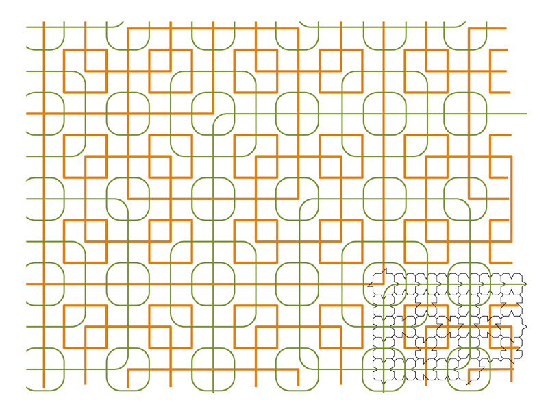
(Credit: Wikimedia)
So, here we do not have triangles but squares, but apart from this it looks very similar to the Sierpinski triangle. Focus on the orange squares: there are some smaller ones, and they are sitting at the corners of slightly larger squares, which are in turn at the corners of even larger squares, and so on. While at a first look it might seem like a periodic pattern, it is not, since larger and larger squares keep appearing. We will come back to this orange squares in a while, keep them in mind.
In 1974, Roger Penrose found a set of just 2 aperiodic tiles, but which are not squares.

Penrose also had this cute idea that one could make a puzzle game out of these shapes, and he even got a patent for that! (“The tiles of the invention may be used to form an instructive game or as a visually attractive floor or wall-covering or the like”). At some point such a puzzle game was actually produced, but it is unfortunately out of production now. If you ever stop by the Newton Institute in Cambridge, UK, they own a copy (and they let you play with it!)

One of the characteristics of Penrose’s tiling is that with it one can obtain patterns with a 5-fold rotational symmetry, which means that you can rotate the tiling by 72°, which is 1/5th of 360°. This is interesting because a beautiful, and elementary, argument from Linear Algebra shows that in periodic tilings you can only get 2-, 3-, 4- or 6-fold symmetries (which corresponds to all n-fold symmetries for which ")

Aperiodicity and Undecidability
Going back to Wang’s problem of whether the tiling problem is decidable: how did Berger prove his undecidability result? There are a lot of technical details he had to take care of, but the essence of his proof was to map each step of adding tiles to an ever-growing tiling, to the steps taken by a computer when running an algorithm (also known as a computer program). Each step of running the algorithm would correspond to instructions on which tile to add next and where. Specifically, Berger was interested in simulating the behavior of a very simple, yet very general computer – a Turing machine.
A Turing machine is basically a model for a machine that can run a particular computer algorithm, reduced to the bare minimum. It comprises of four main ingredients:
- A tape of arbitrary length on which the machine can write (and overwrite) symbols,
- A “head” which
- can read/write one symbol at a time (like a scanner/printer combo)
- can move the tape left/right one position at a time
- can store a finite amount of information (in internal memory)
- A program (table of instructions), which tells the “head” what to do next given the symbol it reads on the tape and the current internal memory state.
- An initial internal state (which tells the “head” how to start moving), as well as a final (halting) internal state (which tells the “head” when to stop).
While being a really simple object, Turing machines are capable of running any computer algorithm, no matter how complex, so they can come in handy when you need something simple and extremely versatile at the same time!

For example, we could have a Turing machine which can only read/write the symbols 0 and 1, has 6 internal states labeled with letters A, B, C, D, E, F, and has the following program:
| & | A | B | C | D | E | F |
| 0 | 1RB | 1RC | 1LD | 1RE | 1LA | H |
| 1 | 1LE | 1RF | 0RB | 0LC | 0RD | 1RC |
Here is how to read this table: Assume the initial state of the machine is A and the tape is filled with the symbol 0. The head of the machine will check the entry in the table corresponding to (0,A) and find the instruction “1RB”, which instructs it to write the symbol 1 (flipping the 0 that was already there to a 1), move the tape to the right, and change the internal state of the head to B. The head will now look up the new instructions for (0,B) (since, after moving the tape to the right, the new symbol under the head will be a 0 again), find “1RC” on the table of instructions, change the 0 into a 1, move the tape to the right once again, and change the internal state to C. It will repeat this process, reading one symbol at a time, checking its table of instructions to decide what to do next, until it reads a 0 while being in state F. If that happens, the special instruction “H” tells the machine to stop its execution: it has reached the “halting” state.
You can try to simulate the execution of this machine on a piece of paper, at least for the first few steps (you might need quite a lot of paper if you want to keep going). Or you could use a computer to simulate it. But you may find that after ten, or a thousand, or a million steps the machine has not halted yet. What if we kept going for another million steps? What about a billion? Can we be sure that the machine will halt eventually?
In his landmark work of 1936, Alan Turing showed that analyzing the behavior of this type of machines is outside the reach of any algorithmic computation: there cannot exist any algorithm which, given the description of a Turing machine’s program, can decide whether the machine will eventually halt, or if the machine will keep running forever! This is known as the halting problem.
Berger’s idea was to simulate a Turing machine using a set of tiles. For each possible symbol, the machine could read or write on the tape, he associated a corresponding color for each edge on the tile borders, as well as one color for each of the possible internal states of the machine. As you can probably guess, for two tiles to be neighbors, their common borders had to have the same color. Then he defined a set of tiles which “implemented” the transitions of the machine’s program, in such a way that each horizontal line was one “time step” of the tape during the execution of the machine. The resulting tiles looked like this, and the rule for the arrow is: two tiles can be next to each other only if the head of each arrow matches with the tail of another arrow.

Imagine we start our tiling with a row describing the initial state of the machine, which means having a “blank tape” (for example, a tape filled with the symbol 0), and one tile where the head of the machine is. It would look like this.

Then there is only one way we can extend this tiling further: for each of the tiles we have put down, there is only one tile that can go on top of that (try to check it yourself!). This is because the Turing Machine only has one possible transition, starting from the symbol 0 and state A. So after we add an extra layer, the pattern looks like this.

And then we repeat. Each time we put down a new tile, there is only one choice possible: we have to respect the transition rules of the Turing Machine, and our tiling will describe the state of the tape at the various steps of the execution.

If the machine halts at some point because it has completed its task, then there will be no way to add new tiles. In order to be sure that we could tile an arbitrarily large area, we would need to know in advance that the Turing machine defined by these tiles (converted into a set of fixed Turing instructions via Berger’s, or Robinson’s mapping) never halted. But, as I mentioned earlier, Turing showed that no algorithm can ever tell us such a thing. Which means you might regret having chosen these tiles for your new bathroom floor (you definitely should have chosen the ones with the flowers instead).
So, why is the aperiodic tiling so important for Berger’s and Robinson’s proofs? We assumed that we started the tiling with a special line, representing the tape in the “blank” state, and this has forced every other choice in the tiling. But using only the alphabet tiles with a single symbol, we get a periodic tiling which can always fill any region! In order to really force our tiling to have a description of the execution of a Turing Machine, we need to guarantee that the tiling is started with that special initialization line. In Robinson’s construction, this is possible using the orange squares as guides (go back and look at the picture of Robinson’s aperiodic tiling if you don’t visualize them), forcing the initialization to happen along the lower edge of each orange square which appears in the pattern. But remember, the Turing machine needs to have access to arbitrarily long segments of tape (we cannot predict how much it will need in case it halts), so we need to have arbitrarily large squares in our tiling. And this means, we really need an aperiodic tiling in order to have all possible tape lengths at our disposition! Any periodic tiling would have restricted the maximum amount of tape the machine could have used before repeating itself.
Tiling a quantum system
You might be wondering: what does all of this have to do with physics (you are, after all, reading the Quantum Frontiers blog and not The IKEA Catalogue 2019). The answer is: tiling problems can be converted into Hamiltonian groundstate energy problems. Think of a square lattice, where to each edge we can assign one of the possible edge configurations of your set of tiles. We can force edges of a square to come from one of the valid tiles by defining a plaquette interaction which gives an energy penalty to non-valid configurations. In this way, we can tile a region of the plane with our set of tiles if and only if this Hamiltonian has a frustration-free groundstate: a groundstate which simultaneously satisfies all the local plaquette constraints, or in other words, one that has zero energy. Deciding whether of not this special kind of groundstate exists is undecidable!
You do not need quantum mechanics for this, as this is a completely classical problem, but you soon realize that the number of possible configurations of the edges in the lattice is arbitrarily large! If you want to write down the matrix which represents this Hamiltonian interaction, you have to resort to larger and larger matrices.
Here is where quantum mechanics comes to the rescue! In a celebrated result, Toby Cubitt, David Pérez-García and Michael Wolf proved that you can have a similar result, this time for the spectral gap of a local Hamiltonian (the problem of deciding whether the spectrum of the Hamiltonian has a constant gap above the groundstate energy), using only a fixed number of local degrees of freedom. Their result is definitely not easy to explain: the first version of the paper was 146 pages long – luckily they managed to simplify it down to 127 pages… But I can try to give a very minimal explanation of how they managed to do this. The key part of their construction is to encode the rules of the Turing machine not directly in the tiling, but in a complex phase (complex number of unit length) which multiplies a certain fixed set of local Hamiltonian terms. They then use the quantum phase estimation algorithm to read off this phase, feeding this input into a Universal Turing Machine (a programmable Turing machine which can simulate any algorithm). In this way, the number of degrees of freedom needed is fixed, and by varying the complex phase mentioned above, they are able to simulate all possible classical Turing machines!
Quantum tiles on a line
Now that we have entered the realms of local Hamiltonian problems, one might wonder if what is going on here is specific to 2 dimensional systems. Clearly, the same phenomena can happen in 3 or more dimensions, since we can simply take multiple slices of 2D systems and stack them on top of each other. But what about 1 dimensional systems? Can we make this construction work on a line?
Interestingly, Wang’s conjecture in 1D is true: every tiling of a line necessarily has a period. Since we are tiling a line, we can think of each tile as essentially a connection between its left-edge color and its right-edge color. Any set of tiles (and associated edge colors) then defines an oriented graph whose vertices are the colors and whose edges are given by the tiles. The rule is again that tiles can be neighbors if their corresponding edges are the same color. The longest (oriented) path we can find in the graph is then the length of the longest segment which can be tiled. It turns out that this length will be infinite if and only if there is a cycle in the graph. In other words, if there is a period.
So we can’t construct aperiodic tilings in 1D, and the tiling problem is decidable. One might be tempted to guess that the same should happen with the spectral gap of local Hamiltonians: We can look at the terms defining the Hamiltonian and decide if a uniform spectral gap exists, as the size of our quantum system increases. After all, in many cases, 1D systems behave “nicely”: we have the DMRG algorithm, polynomial time algorithms for computing groundstates of gapped Hamiltonians, area laws and matrix product state approximations, no thermal phase transitions or topological order, and so on.
But against all odds, in a paper with Johannes Bausch, Toby Cubitt, and David Perez-Garcia, we showed that the spectral gap problem is still undecidable in 1D. How did we get around the lack of aperiodic tilings in 1D?
The key idea was to construct a Hamiltonian whose groundstate would be periodic in the (state of the) spins of an arbitrarily long spin chain, but with a period depending on the halting time of an algorithm (modeled as a Turing machine) encoded (in binary) in the complex phase multiplying each Hamiltonian term. Roughly speaking, this is how we set this up: We partitioned the set of spins into segments. On each segment, we introduced a special Hamiltonian, known as the Feynman-Kitaev history state Hamiltonian, which made sure that the groundstate on that segment was a transcription of the tape during the execution of the classical Turing machine defined by the complex phase (as discussed above).

If at some point the machine has not halted and is running out of tape, so that the segment is not large enough to contain the complete transcription of its execution, then the machine can “push” the delimiter a bit further away, “stealing” some tape space from its neighbor (more technically: the resulting configuration with a larger tape segment is more energetically favorable than the previous one). But once the machine halts, the tape segment shrinks exactly to the minimal size required for the machine to reach its halting state. So, in case the machine halts, the line is divided up into periodic segments, whose length is exactly the optimal length for the machine to halt. If on the other hand the machine does not halt, then the best configuration is the one where there is a unique tape segment, and only one machine running on it.
To recap, the groundstate of this Hamiltonian looks very different depending on whether the Turing machine (encoded in the phase parameter) eventually halts or not. If it does, the groundstate will look periodic, with the period being determined by the halting time. It is therefore a product state, if we think of each segment as a single, huge, particle. If instead the machine never halts, then the groundstate will have a single, very long segment, with a big Kitaev-Feynman history state, which is a highly entangled state.
Even more interestingly, we can set up the different energy scales in the system to behave as follows: for system sizes where the machine has not halted (because it still does not have enough tape to do so, or because it will never do), the single tape segment groudstate has vanishing (but positive) energy, while after it halts, each segment has a small, negative energy. These negative energies in the halting case keep accumulating, so that the thermodynamic groundstate has strictly negative energy density. We can use this difference in energy density between the two cases to construct a “switch”: we introduce two other Hamiltonians to the system (introducing extra local degrees of freedom), one gapped and one gapless. We couple them to everything else we had already set up (the tape segment and the Kitaev-Feynman history state Hamiltonians), in such a way that only one of them controls the low-energy properties of our system. We can set up the switch based on the difference in the energy density in such a way that, before halting, the system is gapped, and it becomes gapless only after the Turing machine has halted (and we cannot predict if this will ever happen!) Hence, the spectral gap is undecidable!
As is the case for 2D system, we need a very large local Hilbert space dimension to make this construction work (so large we did not even care to compute an exact number – but we know it is finite!) On the other extreme end, we know if the local dimension is 2 (we have qubits on a line), and the Hamiltonian has a special property called frustration freeness, then the spectral gap problem is easy to solve. Contrast this with the aperiodic tiling constructions: first Berger found a highly complicated case (with 20,426 tiles), then his construction was refined and simplified over and over, until Robinson got it down to 6 and Penrose showed a similar one with only 2 tiles.
Can we do the same for the undecidability of the spectral gap? At which point does the line become complex enough that the spectral gap problem is undecidable? Can we find some sort of “threshold” which separates the easy and the impossible cases? We need new ideas and new constructions in order to answer all these questions, so let’s get to work!
Comments